神经网络算法是一种受生物神经系统启发而构建的机器学习模型,广泛应用于模式识别、分类、回归等任务。其核心思想是利用大量的简单计算单元(神经元)相互连接形成网络,通过数据学习来实现复杂的非线性映射关系。
神经网络算法是一种受生物神经系统启发而构建的机器学习模型,广泛应用于模式识别、分类、回归等任务。其核心思想是利用大量的简单计算单元(神经元)相互连接形成网络,通过数据学习来实现复杂的非线性映射关系。
神经网络的基本结构
基本构成
神经网络通过调整这些权重,学习输入数据与输出结果之间的映射关系。
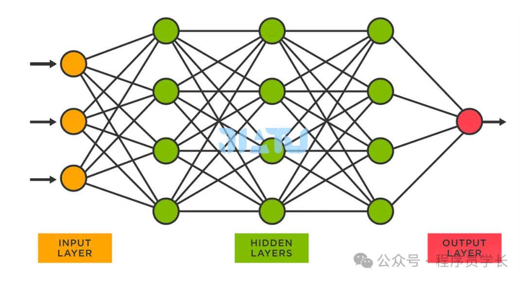
输入层
接收外部数据,每个神经元对应输入数据的一个特征。 隐藏层
位于输入层和输出层之间,负责特征提取和表示。 一个神经网络可以有多个隐藏层,隐藏层的层数和每层神经元数量可以根据具体任务调整。 输出层
生成最终的预测结果,如分类标签或回归值。 神经元数量依据具体任务而定(例如,分类任务中的类别数)。
神经元
每个神经元接收来自前一层神经元的输入信号,通过加权求和后,然后经过一个激活函数,产生输出信号传递到下一层神经元。
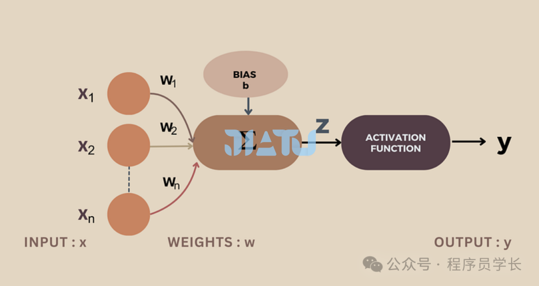
其中:
为输入信号 是对应的权重 b 是偏置 z 为加权和
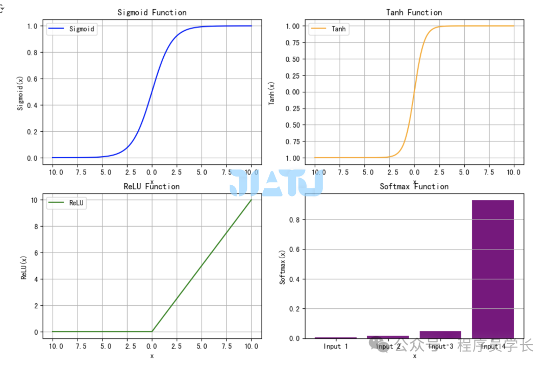
激活函数
Sigmoid 函数
将输入映射到 0 和 1 之间,适合二分类问题输出概率。 Tanh
类似于 Sigmoid,但输出范围中心对称,更适合处理零均值数据。 ReLU
简单高效,对正值保持线性,对负值截断为 0。 Softmax 激活函数
将输入向量转换为概率分布。
import numpy as np
import matplotlib.pyplot as plt

# 定义激活函数
def sigmoid(x):
    return 1 / (1 + np.exp(-x))

def tanh(x):
    return np.tanh(x)

def relu(x):
    return np.maximum(0, x)

def softmax(x):
    e_x = np.exp(x - np.max(x))
    return e_x / e_x.sum(axis=0)


x = np.linspace(-10, 10, 500)
sigmoid_y = sigmoid(x)
tanh_y = tanh(x)
relu_y = relu(x)

softmax_input = np.array([1.0, 2.0, 3.0, 6.0])
softmax_y = softmax(softmax_input)

# 绘制 Sigmoid
plt.figure(figsize=(12, 8))
plt.subplot(2, 2, 1)
plt.plot(x, sigmoid_y, label="Sigmoid", color="blue")
plt.title("Sigmoid Function")
plt.xlabel("x")
plt.ylabel("Sigmoid(x)")
plt.grid()
plt.legend()

# 绘制 Tanh
plt.subplot(2, 2, 2)
plt.plot(x, tanh_y, label="Tanh", color="orange")
plt.title("Tanh Function")
plt.xlabel("x")
plt.ylabel("Tanh(x)")
plt.grid()
plt.legend()

# 绘制 ReLU
plt.subplot(2, 2, 3)
plt.plot(x, relu_y, label="ReLU", color="green")
plt.title("ReLU Function")
plt.xlabel("x")
plt.ylabel("ReLU(x)")
plt.grid()
plt.legend()

# 绘制 Softmax 的柱状图
plt.subplot(2, 2, 4)
categories = [f"Input {i+1}" for i in range(len(softmax_input))]
plt.bar(categories, softmax_y, color="purple")
plt.title("Softmax Function")
plt.xlabel("x")
plt.ylabel("Softmax(x)")
plt.grid(axis="y")
plt.show()
神经网络的训练过程
神经网络的训练过程主要包括前向传播、损失计算、反向传播和参数更新。
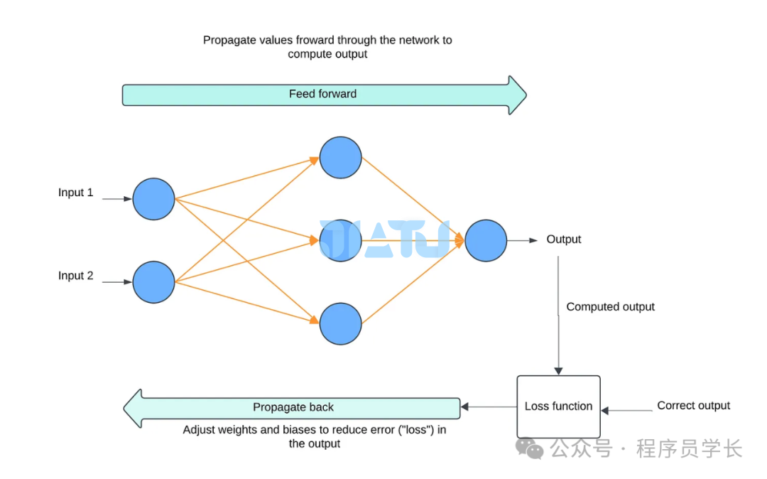
前向传播
其中:
为第 层的权重矩阵 为第 层的激活值 为第 层的偏置向量 为激活函数
损失函数
均方误差 (MSE)
交叉熵损失
用于分类问题。
反向传播和权重更新
输出层误差
首先计算输出层的误差,即损失函数对输出层激活值的偏导数 隐藏层误差
对于隐藏层的神经元,误差由上一层传播过来,通过链式法则计算。 对于第 l 层,误差为: 梯度计算
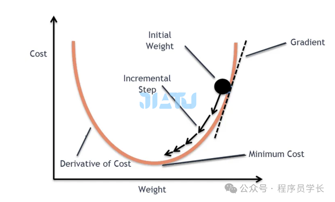
反向传播中,我们计算每一层的权重和偏置的梯度 权重更新
通过反向传播计算得到每一层权重和偏置的梯度后,使用梯度下降法等优化算法来更新参数。 其中, 是学习率,控制每次更新的步长
通过多次迭代前向传播和反向传播,神经网络能够逐步找到最优的权重和偏置,最终实现较高的预测精度。
TensorFlow 实现
import tensorflow as tf
from sklearn.datasets import load_iris
from sklearn.model_selection import train_test_split
from sklearn.preprocessing import StandardScaler, OneHotEncoder
import matplotlib.pyplot as plt
iris = load_iris()
X = iris.data
y = iris.target
scaler = StandardScaler()
X = scaler.fit_transform(X)
encoder = OneHotEncoder(sparse_output=False)
y = encoder.fit_transform(y.reshape(-1, 1))
X_train, X_test, y_train, y_test = train_test_split(X, y, test_size=0.2, random_state=42)
# 构建神经网络模型
model = tf.keras.Sequential([
tf.keras.layers.Dense(16, activation='relu', input_shape=(4,)),
tf.keras.layers.Dense(3, activation='softmax')
])
model.compile(optimizer='adam', loss='categorical_crossentropy', metrics=['accuracy'])
# 训练模型
history = model.fit(X_train, y_train, epochs=100, batch_size=16, validation_data=(X_test, y_test), verbose=1)
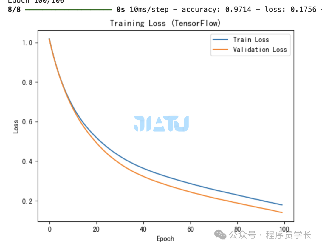
# 绘制损失函数图像
plt.plot(history.history['loss'], label='Train Loss')
plt.plot(history.history['val_loss'], label='Validation Loss')
plt.xlabel('Epoch')
plt.ylabel('Loss')
plt.title('Training Loss (TensorFlow)')
plt.legend()
plt.show()
PyTorch 实现
import torch
import torch.nn as nn
import torch.optim as optim
from sklearn.datasets import load_iris
from sklearn.model_selection import train_test_split
from sklearn.preprocessing import StandardScaler, OneHotEncoder
import matplotlib.pyplot as plt
iris = load_iris()
X = iris.data
y = iris.target
scaler = StandardScaler()
X = scaler.fit_transform(X)
encoder = OneHotEncoder(sparse_output=False)
y = encoder.fit_transform(y.reshape(-1, 1))
X_train, X_test, y_train, y_test = train_test_split(X, y, test_size=0.2, random_state=42)
# 转换为张量
X_train = torch.tensor(X_train, dtype=torch.float32)
X_test = torch.tensor(X_test, dtype=torch.float32)
y_train = torch.tensor(y_train, dtype=torch.float32)
y_test = torch.tensor(y_test, dtype=torch.float32)
# 定义神经网络模型
class NeuralNetwork(nn.Module):
def __init__(self):
super(NeuralNetwork, self).__init__()
self.fc1 = nn.Linear(4, 16)
self.fc2 = nn.Linear(16, 3)
self.relu = nn.ReLU()
def forward(self, x):
x = self.relu(self.fc1(x))
x = self.fc2(x)
return x
model = NeuralNetwork()
# 定义损失函数和优化器
criterion = nn.CrossEntropyLoss()
optimizer = optim.Adam(model.parameters(), lr=0.01)
# 训练模型
losses = []
epochs = 100
for epoch in range(epochs):
optimizer.zero_grad()
outputs = model(X_train)
loss = criterion(outputs, torch.argmax(y_train, axis=1))
loss.backward()
optimizer.step()
losses.append(loss.item())
if (epoch + 1) % 10 == 0:
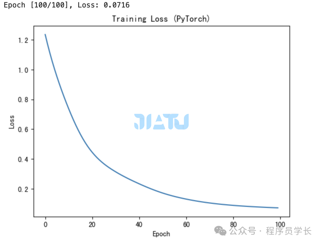
print(f"Epoch [{epoch + 1}/{epochs}], Loss: {loss.item():.4f}")
# 绘制损失函数图像
plt.plot(range(epochs), losses)
plt.xlabel('Epoch')
plt.ylabel('Loss')
plt.title('Training Loss (PyTorch)')
plt.show()